Using statistics
Anaconda Enterprise supports statistical work using the R language and Python libraries such as NumPy, SciPy, Pandas, Statsmodels, and scikit-learn.
The following Jupyter notebook Python examples show how to use these libraries to calculate correlations, distributions, regressions, and principal component analysis.
These examples also include plots produced with the libraries seaborn and Matplotlib.
We thank these sites, from whom we have adapted some code:
Start by importing necessary libraries and functions, including Pandas, SciPy, scikit-learn, Statsmodels, seaborn, and Matplotlib.
This code imports load_boston to provide the Boston housing dataset from the
datasets included with scikit-learn.
import pandas as pd
import seaborn as sns
from scipy.stats import pearsonr
from sklearn.datasets import load_boston
from sklearn.linear_model import LinearRegression
from sklearn.metrics import mean_squared_error
from sklearn.model_selection import train_test_split
from sklearn.preprocessing import StandardScaler
from sklearn.decomposition import PCA
import matplotlib.pyplot as plt
from mpl_toolkits.mplot3d import Axes3D
import statsmodels.formula.api as sm

%matplotlib inline
Load the Boston housing data into a Pandas DataFrame:
#Load dataset and convert it to a Pandas dataframe
boston = load_boston()
df = pd.DataFrame(boston.data, columns=boston.feature_names)
df['target'] = boston.target
In the Boston housing dataset, the target variable is MEDV, the median home value.
Print the dataset description:
#Description of the dataset
print(boston.DESCR)
Boston House Prices dataset
===========================

Notes
------
Data Set Characteristics:

:Number of Instances: 506

:Number of Attributes: 13 numeric/categorical predictive

:Median Value (attribute 14) is usually the target

:Attribute Information (in order):
    - CRIM     per capita crime rate by town
    - ZN       proportion of residential land zoned for lots over 25,000 sq.ft.
    - INDUS    proportion of non-retail business acres per town
    - CHAS     Charles River dummy variable (= 1 if tract bounds river; 0 otherwise)
    - NOX      nitric oxides concentration (parts per 10 million)
    - RM       average number of rooms per dwelling
    - AGE      proportion of owner-occupied units built prior to 1940
    - DIS      weighted distances to five Boston employment centres
    - RAD      index of accessibility to radial highways
    - TAX      full-value property-tax rate per $10,000
    - PTRATIO  pupil-teacher ratio by town
    - B        1000(Bk - 0.63)^2 where Bk is the proportion of blacks by town
    - LSTAT    % lower status of the population
    - MEDV     Median value of owner-occupied homes in $1000's

:Missing Attribute Values: None

:Creator: Harrison, D. and Rubinfeld, D.L.

This is a copy of UCI ML housing dataset.
http://archive.ics.uci.edu/ml/datasets/Housing


This dataset was taken from the StatLib library which is maintained at Carnegie Mellon University.

The Boston house-price data of Harrison, D. and Rubinfeld, D.L. 'Hedonic
prices and the demand for clean air', J. Environ. Economics & Management,
vol.5, 81-102, 1978.   Used in Belsley, Kuh & Welsch, 'Regression diagnostics
...', Wiley, 1980.   N.B. Various transformations are used in the table on
pages 244-261 of the latter.

The Boston house-price data has been used in many machine learning papers that address regression
problems.

**References**

- Belsley, Kuh & Welsch, 'Regression diagnostics: Identifying Influential Data and Sources of Collinearity', Wiley, 1980. 244-261.
- Quinlan,R. (1993). Combining Instance-Based and Model-Based Learning. In Proceedings on the Tenth International Conference of Machine Learning, 236-243, University of Massachusetts, Amherst. Morgan Kaufmann.
- many more! (see http://archive.ics.uci.edu/ml/datasets/Housing)
Show the first five records of the dataset:
#Check the first five records
df.head()
row CRIM    ZN   INDUS CHAS NOX   RM    AGE  DIS    RAD TAX   PTRATIO B      LSTAT target
=== ======= ==== ===== ==== ===== ===== ==== ====== === ===== ======= ====== ===== ======
0   0.00632 18.0 2.31  0.0  0.538 6.575 65.2 4.0900 1.0 296.0 15.3    396.90 4.98  24.0
1   0.02731 0.0  7.07  0.0  0.469 6.421 78.9 4.9671 2.0 242.0 17.8    396.90 9.14  21.6
2   0.02729 0.0  7.07  0.0  0.469 7.185 61.1 4.9671 2.0 242.0 17.8    392.83 4.03  34.7
3   0.03237 0.0  2.18  0.0  0.458 6.998 45.8 6.0622 3.0 222.0 18.7    394.63 2.94  33.4
4   0.06905 0.0  2.18  0.0  0.458 7.147 54.2 6.0622 3.0 222.0 18.7    396.90 5.33  36.2
Show summary statistics for each variable: count, mean, standard deviation, minimum, 25th 50th and 75th percentiles, and maximum.
#Descriptions of each variable
df.describe()
stat  CRIM       ZN         INDUS      CHAS       NOX        RM         AGE        DIS        RAD        TAX        PTRATIO    B          LSTAT      target
===== ========== ========== ========== ========== ========== ========== ========== ========== ========== ========== ========== ========== ========== ==========
count 506.000000 506.000000 506.000000 506.000000 506.000000 506.000000 506.000000 506.000000 506.000000 506.000000 506.000000 506.000000 506.000000 506.000000
mean  3.593761   11.363636  11.136779  0.069170   0.554695   6.284634   68.574901  3.795043   9.549407   408.237154 18.455534  356.674032 12.653063  22.532806
std   8.596783   23.322453  6.860353   0.253994   0.115878   0.702617   28.148861  2.105710   8.707259   168.537116 2.164946   91.294864  7.141062   9.197104
min   0.006320   0.000000   0.460000   0.000000   0.385000   3.561000   2.900000   1.129600   1.000000   187.000000 12.600000  0.320000   1.730000   5.000000
25%   0.082045   0.000000   5.190000   0.000000   0.449000   5.885500   45.025000  2.100175   4.000000   279.000000 17.400000  375.377500 6.950000   17.025000
50%   0.256510   0.000000   9.690000   0.000000   0.538000   6.208500   77.500000  3.207450   5.000000   330.000000 19.050000  391.440000 11.360000  21.200000
75%   3.647423   12.500000  18.100000  0.000000   0.624000   6.623500   94.075000  5.188425   24.000000  666.000000 20.200000  396.225000 16.955000  25.000000
max   88.976200  100.000000 27.740000  1.000000   0.871000   8.780000   100.000000 12.126500  24.000000  711.000000 22.000000  396.900000 37.970000  50.000000
Correlation matrix
The correlation matrix lists the correlation of each variable with each other variable.
Positive correlations mean one variable tends to be high when the other is high, and negative correlations mean one variable tends to be high when the other is low.
Correlations close to zero are weak and cause a variable to have less influence in the model, and correlations close to one or negative one are strong and cause a variable to have more influence in the model.
#Here shows the basic correlation matrix
corr = df.corr()
corr
variable CRIM      ZN        INDUS     CHAS      NOX       RM        AGE       DIS       RAD       TAX       PTRATIO   B         LSTAT     target
======== ========= ========= ========= ========= ========= ========= ========= ========= ========= ========= ========= ========= ========= =========
CRIM     1.000000  -0.199458 0.404471  -0.055295 0.417521  -0.219940 0.350784  -0.377904 0.622029  0.579564  0.288250  -0.377365 0.452220  -0.385832
ZN       -0.199458 1.000000  -0.533828 -0.042697 -0.516604 0.311991  -0.569537 0.664408  -0.311948 -0.314563 -0.391679 0.175520  -0.412995 0.360445
INDUS    0.404471  -0.533828 1.000000  0.062938  0.763651  -0.391676 0.644779  -0.708027 0.595129  0.720760  0.383248  -0.356977 0.603800  -0.483725
CHAS     -0.055295 -0.042697 0.062938  1.000000  0.091203  0.091251  0.086518  -0.099176 -0.007368 -0.035587 -0.121515 0.048788  -0.053929 0.175260
NOX      0.417521  -0.516604 0.763651  0.091203  1.000000  -0.302188 0.731470  -0.769230 0.611441  0.668023  0.188933  -0.380051 0.590879  -0.427321
RM       -0.219940 0.311991  -0.391676 0.091251  -0.302188 1.000000  -0.240265 0.205246  -0.209847 -0.292048 -0.355501 0.128069  -0.613808 0.695360
AGE      0.350784  -0.569537 0.644779  0.086518  0.731470  -0.240265 1.000000  -0.747881 0.456022  0.506456  0.261515  -0.273534 0.602339  -0.376955
DIS      -0.377904 0.664408  -0.708027 -0.099176 -0.769230 0.205246  -0.747881 1.000000  -0.494588 -0.534432 -0.232471 0.291512  -0.496996 0.249929
RAD      0.622029  -0.311948 0.595129  -0.007368 0.611441  -0.209847 0.456022  -0.494588 1.000000  0.910228  0.464741  -0.444413 0.488676  -0.381626
TAX      0.579564  -0.314563 0.720760  -0.035587 0.668023  -0.292048 0.506456  -0.534432 0.910228  1.000000  0.460853  -0.441808 0.543993  -0.468536
PTRATIO  0.288250  -0.391679 0.383248  -0.121515 0.188933  -0.355501 0.261515  -0.232471 0.464741  0.460853  1.000000  -0.177383 0.374044  -0.507787
B        -0.377365 0.175520  -0.356977 0.048788  -0.380051 0.128069  -0.273534 0.291512  -0.444413 -0.441808 -0.177383 1.000000  -0.366087 0.333461
LSTAT    0.452220  -0.412995 0.603800  -0.053929 0.590879  -0.613808 0.602339  -0.496996 0.488676  0.543993  0.374044  -0.366087 1.000000  -0.737663
target   -0.385832 0.360445  -0.483725 0.175260  -0.427321 0.695360  -0.376955 0.249929  -0.381626 -0.468536 -0.507787 0.333461  -0.737663 1.000000
Format with asterisks
Format the correlation matrix by rounding the numbers to two decimal places and adding asterisks to denote statistical significance:
def calculate_pvalues(df):
    df = df.select_dtypes(include=['number'])
    pairs = pd.MultiIndex.from_product([df.columns, df.columns])
    pvalues = [pearsonr(df[a], df[b])[1] for a, b in pairs]
    pvalues = pd.Series(pvalues, index=pairs).unstack().round(4)
    return pvalues

# code adapted from https://stackoverflow.com/questions/25571882/pandas-columns-correlation-with-statistical-significance/49040342
def correlation_matrix(df,columns):
    rho = df[columns].corr()
    pval = calculate_pvalues(df[columns])
    # create three masks
    r0 = rho.applymap(lambda x: '{:.2f}'.format(x))
    r1 = rho.applymap(lambda x: '{:.2f}*'.format(x))
    r2 = rho.applymap(lambda x: '{:.2f}**'.format(x))
    r3 = rho.applymap(lambda x: '{:.2f}***'.format(x))
    # apply marks
    rho = rho.mask(pval>0.01,r0)
    rho = rho.mask(pval<=0.1,r1)
    rho = rho.mask(pval<=0.05,r2)
    rho = rho.mask(pval<=0.01,r3)
    return rho

columns = df.columns
correlation_matrix(df,columns)
variable CRIM     ZN       INDUS    CHAS     NOX      RM       AGE      DIS      RAD      TAX      PTRATIO  B        LSTAT    target
======== ======== ======== ======== ======== ======== ======== ======== ======== ======== ======== ======== ======== ======== ========
CRIM     1.00***  -0.20*** 0.40***  -0.06    0.42***  -0.22*** 0.35***  -0.38*** 0.62***  0.58***  0.29***  -0.38*** 0.45***  -0.39***
ZN       -0.20*** 1.00***  -0.53*** -0.04    -0.52*** 0.31***  -0.57*** 0.66***  -0.31*** -0.31*** -0.39*** 0.18***  -0.41*** 0.36***
INDUS    0.40***  -0.53*** 1.00***  0.06     0.76***  -0.39*** 0.64***  -0.71*** 0.60***  0.72***  0.38***  -0.36*** 0.60***  -0.48***
CHAS     -0.06    -0.04    0.06     1.00***  0.09**   0.09**   0.09*    -0.10**  -0.01    -0.04    -0.12*** 0.05     -0.05    0.18***
NOX      0.42***  -0.52*** 0.76***  0.09**   1.00***  -0.30*** 0.73***  -0.77*** 0.61***  0.67***  0.19***  -0.38*** 0.59***  -0.43***
RM       -0.22*** 0.31***  -0.39*** 0.09**   -0.30*** 1.00***  -0.24*** 0.21***  -0.21*** -0.29*** -0.36*** 0.13***  -0.61*** 0.70***
AGE      0.35***  -0.57*** 0.64***  0.09*    0.73***  -0.24*** 1.00***  -0.75*** 0.46***  0.51***  0.26***  -0.27*** 0.60***  -0.38***
DIS      -0.38*** 0.66***  -0.71*** -0.10**  -0.77*** 0.21***  -0.75*** 1.00***  -0.49*** -0.53*** -0.23*** 0.29***  -0.50*** 0.25***
RAD      0.62***  -0.31*** 0.60***  -0.01    0.61***  -0.21*** 0.46***  -0.49*** 1.00***  0.91***  0.46***  -0.44*** 0.49***  -0.38***
TAX      0.58***  -0.31*** 0.72***  -0.04    0.67***  -0.29*** 0.51***  -0.53*** 0.91***  1.00***  0.46***  -0.44*** 0.54***  -0.47***
PTRATIO  0.29***  -0.39*** 0.38***  -0.12*** 0.19***  -0.36*** 0.26***  -0.23*** 0.46***  0.46***  1.00***  -0.18*** 0.37***  -0.51***
B        -0.38*** 0.18***  -0.36*** 0.05     -0.38*** 0.13***  -0.27*** 0.29***  -0.44*** -0.44*** -0.18*** 1.00***  -0.37*** 0.33***
LSTAT    0.45***  -0.41*** 0.60***  -0.05    0.59***  -0.61*** 0.60***  -0.50*** 0.49***  0.54***  0.37***  -0.37*** 1.00***  -0.74***
target   -0.39*** 0.36***  -0.48*** 0.18***  -0.43*** 0.70***  -0.38*** 0.25***  -0.38*** -0.47*** -0.51*** 0.33***  -0.74*** 1.00***
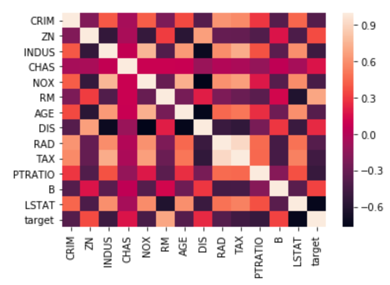
Heatmap
Heatmap of the correlation matrix:
sns.heatmap(corr,
        xticklabels=corr.columns,
        yticklabels=corr.columns)
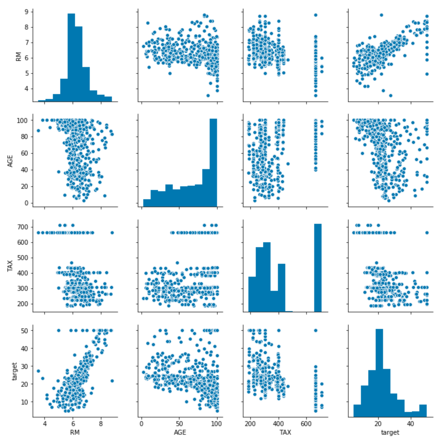
Pairwise distributions with seaborn
sns.pairplot(df[['RM', 'AGE', 'TAX', 'target']])
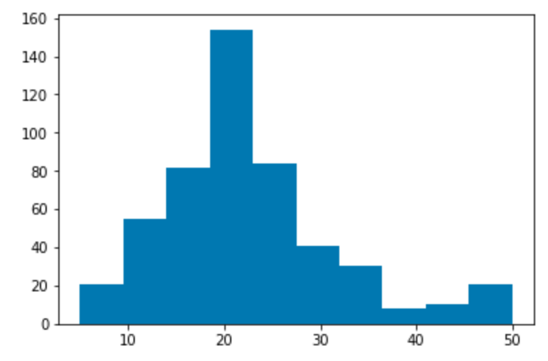
Target variable distribution
Histogram showing the distribution of the target variable. In this dataset this is “Median value of owner-occupied homes in $1000’s”, abbreviated MEDV.
plt.hist(df['target'])
plt.show()
Simple linear regression
The variable MEDV is the target that the model predicts. All other variables are used as predictors, also called features.
The target variable is continuous, so use a linear regression instead of a logistic regression.
# Define features as X, target as y.
X = df.drop('target', axis='columns')
y = df['target']
Split the dataset into a training set and a test set:
# Splitting the dataset into training set and test set
X_train, X_test, y_train, y_test = train_test_split(X, y, test_size = 0.25, random_state = 0)
A linear regression consists of a coefficient for each feature and one intercept.
To make a prediction, each feature is multiplied by its coefficient. The intercept and all of these products are added together. This sum is the predicted value of the target variable.
The residual sum of squares (RSS) is calculated to measure the difference between the prediction and the actual value of the target variable.
The function fit calculates the coefficients and intercept that minimize the
RSS when the regression is used on each record in the training set.
# Fitting Simple Linear Regression to the Training set
from sklearn.linear_model import LinearRegression
regressor = LinearRegression()
regressor.fit(X_train, y_train)

# The intercept
print('Intercept: \n', regressor.intercept_)

# The coefficients
print('Coefficients: \n', pd.Series(regressor.coef_, index=X.columns, name='coefficients'))
Intercept:
 36.98045533762056
Coefficients:
 CRIM       -0.116870
ZN          0.043994
INDUS      -0.005348
CHAS        2.394554
NOX       -15.629837
RM          3.761455
AGE        -0.006950
DIS        -1.435205
RAD         0.239756
TAX        -0.011294
PTRATIO    -0.986626
B           0.008557
LSTAT      -0.500029
Name: coefficients, dtype: float64
Now check the accuracy when this linear regression is used on new data that it was not trained on. That new data is the test set.
# Predicting the Test set results
y_pred = regressor.predict(X_test)

# Visualising the Test set results
# code adapted from https://joomik.github.io/Housing/
fig, ax = plt.subplots()
ax.scatter(y_test, y_pred, color='green')
ax.set(
    xlabel="Prices: $Y_i$",
    ylabel="Predicted prices: $\hat{Y}_i$",
    title="Prices vs Predicted prices: $Y_i$ vs $\hat{Y}_i$",
)
plt.show()
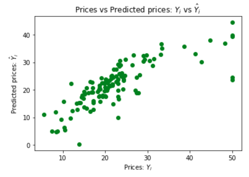
This scatter plot shows that the regression is a good predictor of the data in the test set.
The mean squared error quantifies this performance:
# The mean squared error as a way to measure model performance.
print("Mean squared error: %.2f" % mean_squared_error(y_test, y_pred))
Mean squared error: 29.79
Ordinary least squares (OLS) regression with Statsmodels
model = sm.ols('target ~ AGE + B + CHAS + CRIM + DIS + INDUS + LSTAT + NOX + PTRATIO + RAD + RM + TAX + ZN', df)
result = model.fit()
result.summary()
OLS Regression Results
==============================================================================
Dep. Variable:                 target   R-squared:                       0.741
Model:                            OLS   Adj. R-squared:                  0.734
Method:                 Least Squares   F-statistic:                     108.1
Date:                Thu, 23 Aug 2018   Prob (F-statistic):          6.95e-135
Time:                        07:29:16   Log-Likelihood:                -1498.8
No. Observations:                 506   AIC:                             3026.
Df Residuals:                     492   BIC:                             3085.
Df Model:                          13
Covariance Type:            nonrobust
==============================================================================
coef    std err          t      P>|t|      [0.025      0.975]
------------------------------------------------------------------------------
Intercept     36.4911      5.104      7.149      0.000      26.462      46.520
AGE            0.0008      0.013      0.057      0.955      -0.025       0.027
B              0.0094      0.003      3.500      0.001       0.004       0.015
CHAS           2.6886      0.862      3.120      0.002       0.996       4.381
CRIM          -0.1072      0.033     -3.276      0.001      -0.171      -0.043
DIS           -1.4758      0.199     -7.398      0.000      -1.868      -1.084
INDUS          0.0209      0.061      0.339      0.735      -0.100       0.142
LSTAT         -0.5255      0.051    -10.366      0.000      -0.625      -0.426
NOX          -17.7958      3.821     -4.658      0.000     -25.302     -10.289
PTRATIO       -0.9535      0.131     -7.287      0.000      -1.211      -0.696
RAD            0.3057      0.066      4.608      0.000       0.175       0.436
RM             3.8048      0.418      9.102      0.000       2.983       4.626
TAX           -0.0123      0.004     -3.278      0.001      -0.020      -0.005
ZN             0.0464      0.014      3.380      0.001       0.019       0.073
==============================================================================
Omnibus:                      178.029   Durbin-Watson:                   1.078
Prob(Omnibus):                  0.000   Jarque-Bera (JB):              782.015
Skew:                           1.521   Prob(JB):                    1.54e-170
Kurtosis:                       8.276   Cond. No.                     1.51e+04
==============================================================================

Warnings:
[1] Standard Errors assume that the covariance matrix of the errors is correctly specified.
[2] The condition number is large, 1.51e+04. This might indicate that there are
strong multicollinearity or other numerical problems.
Principal component analysis
The initial dataset has a number of feature or predictor variables and one target variable to predict.
Principal component analysis (PCA) converts these features into a set of principal components, which are linearly uncorrelated variables.
The first principal component has the largest possible variance and therefore accounts for as much of the variability in the data as possible.
Each of the other principal components is orthogonal to all of its preceding components, but has the largest possible variance within that constraint.
Graphing a dataset by showing only the first two or three of the principal components effectively projects a complex dataset with high dimensionality into a simpler image that shows as much of the variance in the data as possible.
PCA is sensitive to the relative scaling of the original variables, so begin by scaling them:
# Feature Scaling
x = StandardScaler().fit_transform(X)
Calculate the first three principal components and show them for the first five rows of the housing dataset:
# Project data to 3 dimensions
pca = PCA(n_components=3)
principalComponents = pca.fit_transform(x)
principalDf = pd.DataFrame(
    data = principalComponents,
    columns = ['principal component 1', 'principal component 2', 'principal component 3'])
principalDf.head()
row |
principal component 1 |
principal component 2 |
principal component 3 |
|---|---|---|---|
0 |
-2.097842 |
0.777102 |
0.335076 |
1 |
-1.456412 |
0.588088 |
-0.701340 |
2 |
-2.074152 |
0.602185 |
0.161234 |
3 |
-2.611332 |
-0.005981 |
-0.101940 |
4 |
-2.457972 |
0.098860 |
-0.077893 |
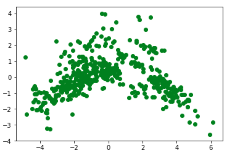
Show a 2D graph of this data:
plt.scatter(principalDf['principal component 1'], principalDf['principal component 2'], color ='green')
plt.show()
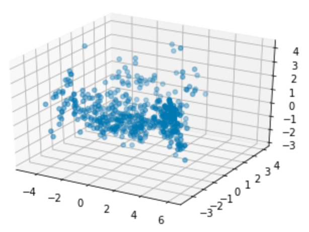
Show a 3D graph of this data:
fig = plt.figure()
ax = fig.add_subplot(111, projection='3d')
ax.scatter(principalDf['principal component 1'], principalDf['principal component 2'], principalDf['principal component 3'])
plt.show()
Measure how much of the variance is explained by each of the three components:
# Variance explained by each component
explained_variance = pca.explained_variance_ratio_
explained_variance
array([0.47097344, 0.11015872, 0.09547408])
Each value will be less than or equal to the previous value, and each value will be in the range from 0 through 1.
The sum of these three values shows the fraction of the total variance explained by the three principal components, in the range from 0 (none) through 1 (all):
sum(explained_variance)
0.6766062376563704
Predict the target variable using only the three principal components:
y_test_linear = y_test
y_pred_linear = y_pred
X = principalDf
y = df['target']
X_train, X_test, y_train, y_test = train_test_split(X, y, test_size = 0.25, random_state = 0)
regressor = LinearRegression()
regressor.fit(X_train, y_train)
y_pred = regressor.predict(X_test)
Plot the predictions from the linear regression in green again, and the new predictions in blue:
fig, ax = plt.subplots()
ax.scatter(y_test, y_pred, color='skyblue')
ax.scatter(y_test_linear, y_pred_linear, color = 'green')
ax.set(
    xlabel="Prices: $Y_i$",
    ylabel="Predicted prices: $\hat{Y}_i$",
    title="Prices vs Predicted prices: $Y_i$ vs $\hat{Y}_i$",
)
plt.show()
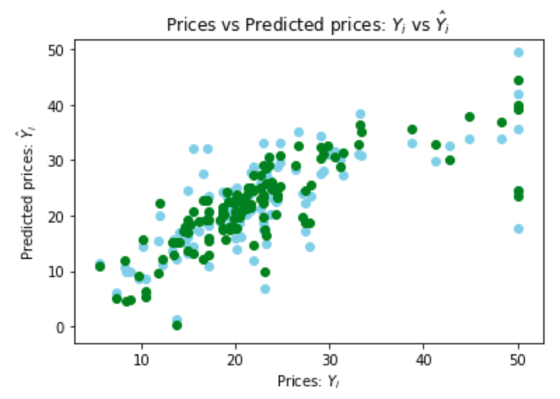
The blue points are somewhat more widely scattered, but similar.
Calculate the mean squared error:
print("Linear regression mean squared error: %.2f" % mean_squared_error(y_test_linear, y_pred_linear))
print("PCA mean squared error: %.2f" % mean_squared_error(y_test, y_pred))
Linear regression mean squared error: 29.79
PCA mean squared error: 43.49